Making figures for microbial ecology: Interactive bar plots

This is the first of several tutorials I’m putting together for making figures that are common in microbial ecology. Today we’ll start with an interactive bar plot for exploring your microbial community data. For this tutorial I’m using data and code from my publication in Geobiology. You can fork the repo by clicking the button above!

To generate the data, we sequenced DNA from microbial communities at our study site DeMMO. The raw sequence data was processed with QIIME to produce an OTU table. OTUs, or operational taxonomic units, are bins that differentiate sequences at a 97% similarity threshold. For our purposes, you can think of an OTU as a species of bacteria or archaea. As a microbial ecologist, you might want to compare the taxonomic compositions of your communities. Let’s make a cool html bar plot to explore our microbial community data!

Before we get started, you’ll need to set up your environment in R. This code depends on the packages being loaded here:

#load libraries 
pacman::p_load(tidyverse, plotly, randomcoloR)

Next, read the OTU data into a dataframe. We can pull the data directy from Github by reading the raw file. You can preview the data in the table below this code chunk.

#read the data into a dataframe
otu_table <- read_delim("https://raw.githubusercontent.com/CaitlinCasar/Casar2020_DeMMO_MineralHostedBiofilms/master/orig_data/DeMMO136_Dec2015toApril2018_noChimera_otuTable_withTaxa_d10000.txt", delim="\t", comment = "# ")
metadata <- read_csv("https://raw.githubusercontent.com/CaitlinCasar/Casar2020_DeMMO_MineralHostedBiofilms/master/orig_data/metadata.csv") 

#store the taxonomy for each OTU
taxonomy <- otu_table %>%
  select(`#OTU ID`, taxonomy) %>%
  mutate(tax = gsub("Gammaproteobacteria; D_3__Betaproteobacteriales", "Betaproteobacteria; D_3__Betaproteobacteriales", taxonomy), #fix taxonomy for Beta's,
         taxonomy = str_remove_all(tax, "D_0__| D_1__| D_2__| D_3__| D_4__| D_5__| D_6__")) %>%
  separate(taxonomy ,sep=';',c("domain", "phylum", "class", "order", "family", "genus", "species")) %>%
  gather(level, taxonomy, domain:species)

We want to look at the community compositions, so first let’s normalize and reshape the data.

abundance_table <- otu_table %>%
  select(-taxonomy) %>%
  mutate_at(vars(-`#OTU ID`), funs(./sum(.)*100)) %>% #normalize to relative abundance 
  gather(sample_id, abundance, `7.DeMMO1.Steri.050917`:`18.800.DitchFluid.041818`) 

For plotting purposes, let’s pick a subset of samples.

barplot_samples <- c("12.DeMMO1.steri.041818", 
                     "26.DeMMO1.SC1.top.041818", 
                     "22.DeMMO1.C.top.041818",
                     "23.DeMMO1.D.top.041818", 
                     "24.DeMMO1.E.top.041818",
                     "27.DeMMO1.SC2.top.041818", 
                     "34.DeMMO1.SC10.top.041818", 
                     "45.DeMMO1.7.top.041818",
                     "46.DeMMO1.8.top.041818", 
                     "47.DeMMO1.9.top.041818",
                     "14.DeMMO3.steri.041718", 
                     "51.DeMMO3.A.top.041718",
                     "27.DeMMO3.T8.top.051117", 
                     "53.DeMMO3.C.top.041718", 
                     "54.DeMMO3.D.top.041718",
                     "55.DeMMO3.E.top.041718", 
                     "39.DeMMO3.1.top.041718", 
                     "40.DeMMO3.2.top.041718",
                     "41.DeMMO3.3.top.041718", 
                     "56.DeMMO3.F.top.041718",
                     "12.DeMMO6.Steri#2.051017", 
                     "13.DeMMO6.T1.top.051017",
                     "15.DeMMO6.T2.top.051017", 
                     "17.DeMMO6.T3.top.051017",
                     "19.DeMMO6.T4.top.051017",
                     "21.DeMMO6.T5.top.051017", 
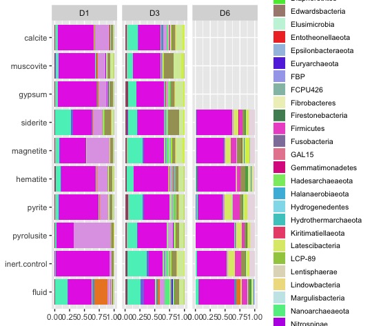
                     "24.DeMMO6.T6.bottom.051017") 

Now, let’s take a look at the phylum level abundances for each sample.

taxon_abundance_table <- abundance_table %>%
  left_join(taxonomy) %>%
  filter(sample_id %in% barplot_samples & level == "phylum") %>%
  mutate(taxonomy = if_else(is.na(taxonomy), "Unassigned", taxonomy))

Let’s make a custom color palette for our phyla.

phylum_color <- distinctColorPalette(k = length(unique(taxon_abundance_table$taxonomy)))
names(phylum_color) <- unique(taxon_abundance_table$taxonomy)

And now, let’s create a stacked bar plot for each site.

bar_plot <- taxon_abundance_table %>%
  left_join(metadata) %>%
  group_by(site, experiment.type, taxonomy) %>%
  summarise(abundance = sum(abundance)) %>%
  ungroup() %>%
  mutate(experiment.type = factor(experiment.type, levels = c("fluid", "inert.control", "pyrolusite", "pyrite","hematite","magnetite","siderite","gypsum","muscovite","calcite"))) %>%
  ggplot(aes(fill=taxonomy, y=abundance, x=experiment.type)) +
  geom_bar(stat='identity', position='fill') +
  scale_fill_manual(values=phylum_color) +
  coord_flip() + 
  theme(axis.title = element_blank(),
        legend.title = ggplot2::element_blank(), 
        legend.text = ggplot2::element_text(size = 8),
        legend.key.size = unit(0.5, "cm")) +
  facet_grid(cols = vars(site), switch = "y") + 
  guides(fill = guide_legend(ncol = 1))

Finally, let’s make it easier to explore our data with an html version of our bar plot!

ggplotly(bar_plot)

Ta da! You now have an interactive html version of your plot that you can view in your web browser - just double click the file in your file explorer and it will automatically open. These files are portable, so you can email them to your collaborators and explore the data together. Stay tuned for upcoming tutorials on making figures for microbial ecology!